Extending the phase test beyond steady tones#
The current app asks whether two periodic tones with the same harmonic amplitudes but different harmonic phases sound the same. A general sound, a drum hit or a spoken word, has no fixed set of harmonics, so "keep the amplitudes, change the phases" needs a new definition. The natural candidate is the spectrogram: at each time and frequency there is a magnitude and a phase, and we would like to keep every magnitude and change the phases. This document explains why that cannot be done literally, describes a formulation that is exact and easy to implement, shows what it does to a click and to a tone, and proposes how to build it into the app. The figures were generated by make_figures.py in this directory and can be regenerated with python3 docs/make_figures.py.
The document is organized as follows. Section 1 fixes terminology. Section 2 shows what goes wrong when phases are changed cell by cell. Section 3 introduces the filter bank view, which is the STFT with a hop of one sample, and Section 4 defines the proposed operation on it. Sections 5 and 6 work out what the operation means for constant and for time-varying phase offsets, because both have well studied perceptual consequences. Section 7 proposes the app design and Section 8 lists open questions.
1. Terminology: the STFT, the spectrogram, and the inverse#
The short-time Fourier transform (STFT) multiplies the signal by a window centered at time t, takes the Fourier transform of the product, and repeats for a grid of window positions spaced by the hop. The windows overlap when the hop is shorter than the window. Each windowed transform gives one column of complex coefficients X(t, f). The spectrogram is the magnitude |X(t, f)|, so strictly speaking the spectrogram has no phase; the object we want to modify is the STFT. With Gaussian windows the STFT is also called the Gabor transform. Figure 1 shows the test signal used throughout, a click followed by a harmonic tone at 220 Hz with eight harmonics of amplitude 1/k, together with the Gaussian windows and the spectrogram.
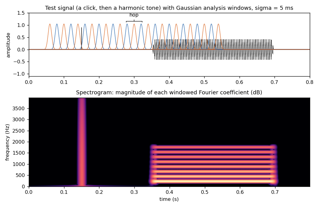
Figure 1. Top: the test signal with Gaussian analysis windows of width sigma = 5 ms, spaced by the hop. Bottom: the spectrogram, the magnitude of the windowed Fourier coefficients.
The inverse STFT (ISTFT) transforms each column back to a windowed piece of signal and adds the pieces, a procedure called overlap-add. The loop "STFT, modify, ISTFT" is what the phase vocoder literature calls analysis-modification-synthesis. The key fact about the STFT is that it is redundant: with a hop of one quarter of the window length there are four times as many complex coefficients as there are real samples. Only a small subset of all possible coefficient arrays are actually the STFT of some signal. Such arrays are called consistent. When a modified array is not consistent, the ISTFT does not fail; it returns the signal whose STFT is closest in the least-squares sense (Griffin and Lim, 1984), and the STFT of that signal differs from the array we asked for.
2. Why phases cannot be changed cell by cell#
Figure 2 makes the consistency problem concrete. We compute a hop-based STFT of the test signal (Hann window, 32 ms, 75% overlap), multiply every coefficient by a random unit phasor, leaving every magnitude untouched, and invert. The recomputed spectrogram of the result is not the original spectrogram. The click has become a burst of noise spread over the window length and the tone has become a noisy band with the right long-term average but a fluctuating envelope. In the right column we instead multiply each frequency bin by one phasor that is the same in every frame. The spectrogram then survives almost unchanged, and the only visible difference is that the click is slightly smeared in time.
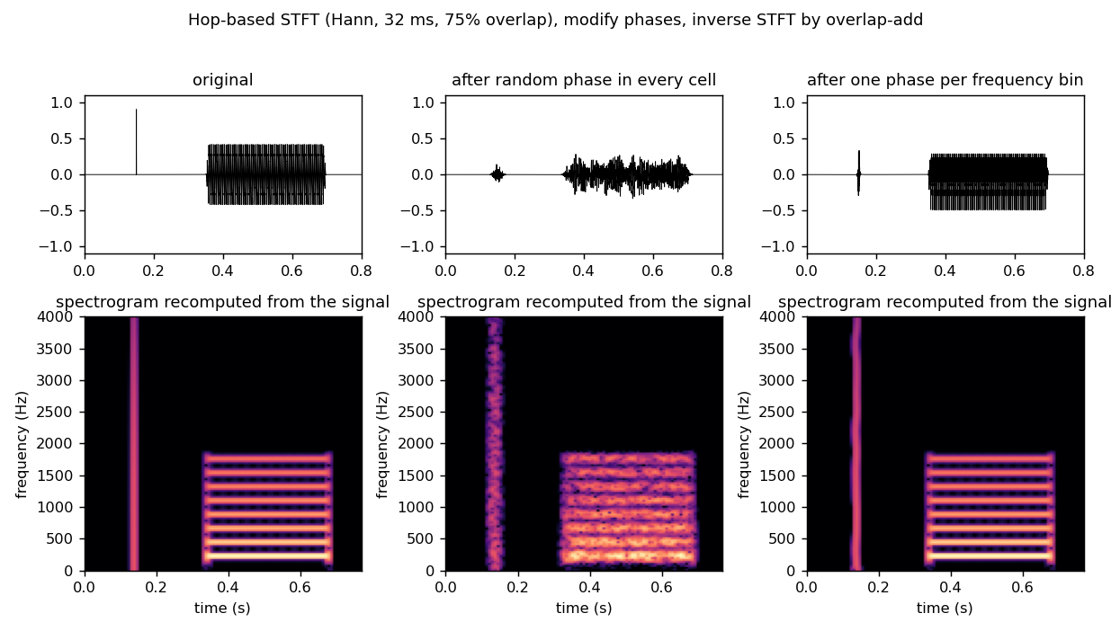
Figure 2. Left: original. Middle: after replacing the phase of every STFT cell by a random value and inverting; the magnitudes were untouched before inversion, but the inversion changes them. Right: after applying one phase per frequency bin, constant across frames.
The reason is that overlapping windows see the same samples, so the phases in neighbouring columns are tied together. A steady sinusoid at frequency f advances its phase by exactly 2 pi f times the hop from one column to the next. Random phases break this relation, the overlapping pieces no longer add coherently, and the ISTFT averages them into something else. Indeed, for a sufficiently redundant STFT the magnitudes alone determine the signal up to a global sign, which is why algorithms such as Griffin-Lim can reconstruct audio from a spectrogram. In that strict sense there is no such thing as "the same spectrogram with different phases". What we can do is preserve the magnitudes at the resolution of the analysis, and this turns out to be the useful question anyway.
3. The filter bank view: a hop of one sample#
Rather than thinking of the STFT as a grid of windowed transforms, we think of it as a bank of filters. Fix a frequency f_k and consider the STFT coefficient at that frequency as a function of the window position t. It equals the convolution of the signal with h_k(t) = w(t) exp(2 pi i f_k t), a bandpass filter with a Gaussian frequency response centered at f_k. We write z_k(t) for this complex subband signal. Evaluating it at every sample, that is, using a hop of one sample, gives a row of the STFT at full time resolution. Its magnitude |z_k(t)| is the subband envelope and its argument is the subband phase.
The frequency responses of the bank overlap heavily (Figure 3, top). We normalize them so that they sum to one at every frequency. Then the original signal is recovered by simply adding the subbands, x(t) = Re sum_k z_k(t), with no overlap-add in time at all. (The negative frequencies are folded in by doubling the positive ones first, the usual analytic-signal convention.) In the figures the bank uses a spacing between centers equal to the Gaussian width sigma_f = 1 / (2 pi sigma), so a 5 ms window gives about 32 Hz spacing and about 250 bands up to the 8 kHz Nyquist frequency of the 16 kHz test signal.
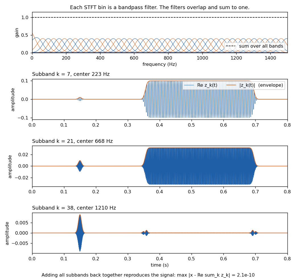
Figure 3. Top: the frequency responses of the bands for sigma = 5 ms, and their sum. Below: three subbands of the test signal, one on the fundamental, one on the third harmonic, one between harmonics. The click appears in every band; each harmonic appears in the bands near its frequency.
This is a standard reformulation, sometimes called the filter bank summation view of the phase vocoder, and it dissolves the question of consistency between overlapping windows. There are no separate windows to keep consistent, only subband signals that are added.
4. The proposed operation: rotate the phase of each subband#
Here we propose to define the phase-modified sound as
y(t) = Re sum_k exp(i phi_k(t)) z_k(t)
where phi_k(t) is the phase offset applied to band k at time t. Every subband envelope |z_k(t)| is exactly unchanged and every subband phase is shifted by exactly the requested amount, at every sample. When phi = 0 we get y = x exactly. This is a direct generalization of what the app does now: for a steady tone whose harmonics are separated by more than the bandwidth, each harmonic lives in its own group of bands, and rotating those bands by a common angle rotates that harmonic's phase.
Figure 4 shows the effect on the test signal for three window widths, using a random phase map that varies smoothly across bands (the reason for the smoothness is given in Section 5). The steady tone keeps its period and its amplitude and only changes waveform shape, which is the situation the current app tests. The click spreads out over roughly the window length: a fraction of a millisecond for sigma = 0.5 ms, tens of milliseconds for sigma = 20 ms. This asymmetry between steady and transient sounds is the central new element the extension brings in.
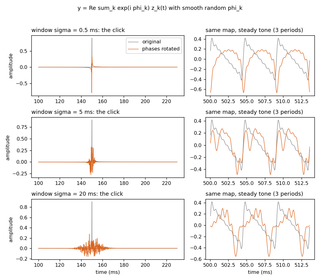
Figure 4. Left: the click before and after phase rotation, for three window widths. Right: three periods of the tone. The steady tone changes shape but not envelope; the click is smeared over the window.
Figure 5 shows what "same spectrogram" means in this setting. Analysed with the same 20 ms window that was used to modify it, the modified signal has essentially the original spectrogram (the click column is a little mottled because different bands were delayed by different amounts within the window). Analysed with a 2 ms window, the original click is a sharp line while the modified click is visibly spread in time. The magnitudes are preserved at the resolution of the analysis and not at finer resolution, and this is unavoidable for the reasons of Section 2.
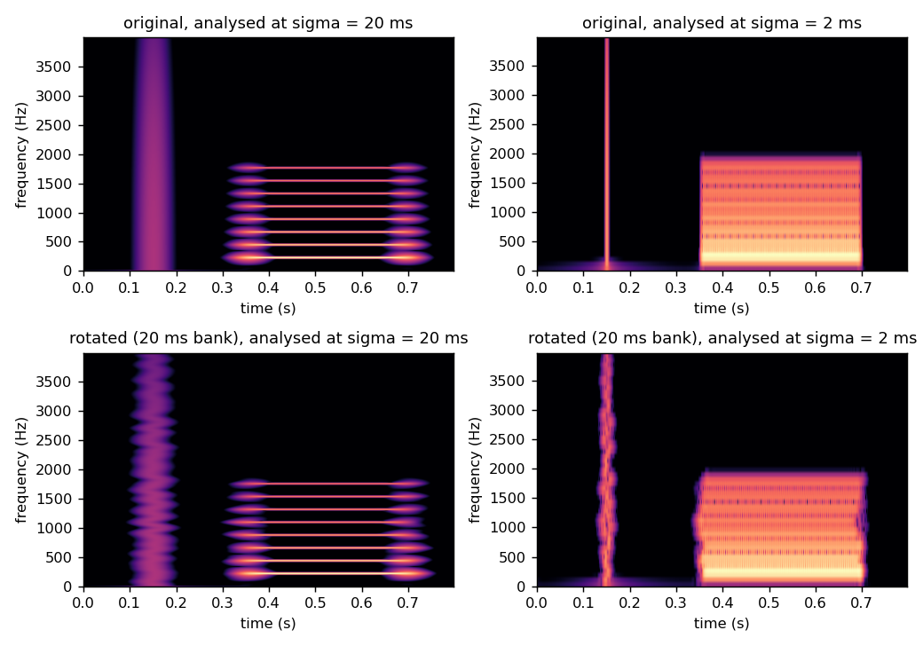
Figure 5. Spectrograms of the original (top) and of the modified signal from the 20 ms bank (bottom), analysed at sigma = 20 ms (left) and at sigma = 2 ms (right).
5. Constant phase offsets are an all-pass filter#
When the offsets do not depend on time, the operation is linear and time-invariant, so it is a filter, and its frequency response is G(f) = sum_k exp(i phi_k) H_k(f) where H_k is the response of band k. Figure 6 plots the magnitude, phase, and group delay of G for the three maps of Figure 4. The group delay is minus the derivative of the phase with respect to angular frequency, tau(f) = -(1 / 2 pi) d phi / d f, and it measures how much the energy near frequency f is delayed by the filter. If the phase varies smoothly across the bands, the magnitude stays within about a decibel of unity and the filter is close to an all-pass filter: it preserves the long-term magnitude spectrum exactly the way the tone app preserves the harmonic amplitudes.
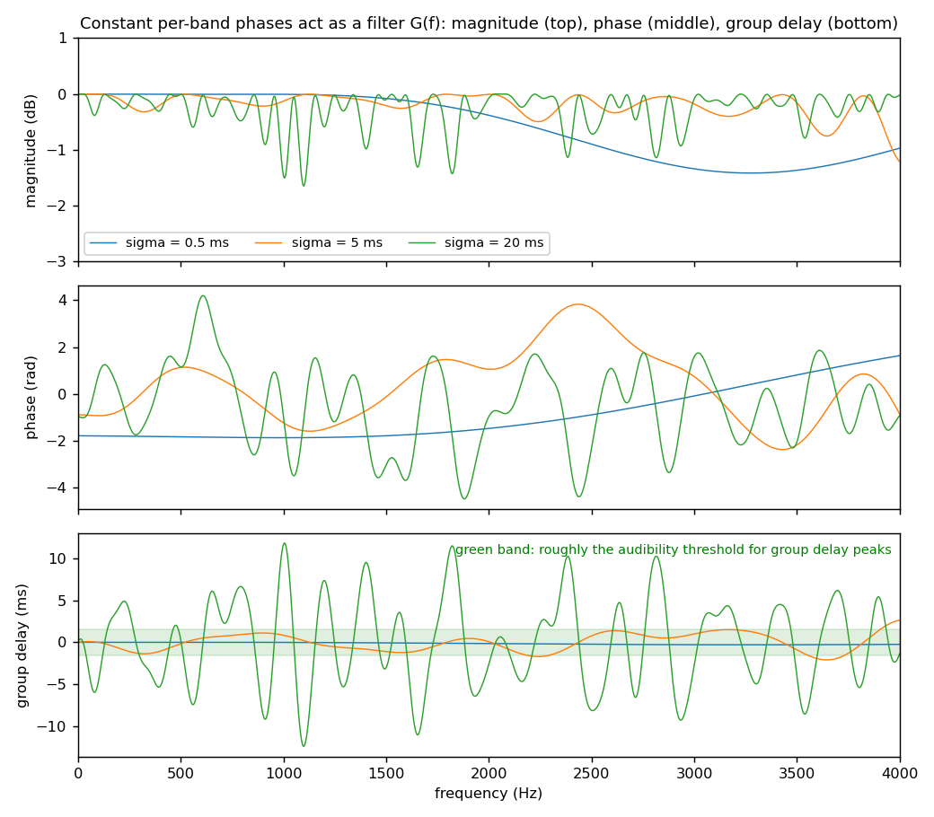
Figure 6. The filter implied by constant per-band phases, for the three window widths of Figure 4. The group delay grows with the window width. The green band marks the approximate audibility threshold for group delay peaks.
The group delay is what makes the click spread. The phase change from one band to the next, divided by the band spacing, sets the delay, and because the spacing scales as 1 / sigma, a random map with a given roughness has a group delay proportional to the window width. Whether a listener can hear this is a well studied question, because all-pass filters occur in loudspeaker crossovers and equalizers. Blauert and Laws (1978) measured thresholds for group delay peaks of about 0.5 to 2 ms depending on frequency, with the lowest thresholds near 2 kHz and with impulsive signals over headphones; steady signals are much less sensitive. The prediction for our experiment is therefore concrete: constant random phase maps should be inaudible on sustained sounds for any window, inaudible on transients for windows below a millisecond or so, and audible as a softening or smearing of transients for windows of several milliseconds and beyond. The tone results already obtained, including the audibility at low fundamentals, are the sustained-sound end of this picture.
One requirement follows from the overlap of the bands: the phase map must vary smoothly from band to band. Figure 7 shows why. Where two neighbouring bands have very different phases, their contributions partly cancel at the frequencies they share, and the magnitude response acquires notches of many decibels. A harmonic of the tone that falls on such a notch is attenuated, which changes the amplitude spectrum and defeats the purpose of the test. Smoothing the random map over a handful of bands removes the notches while leaving the group delay large. (An independent random phase per band is the analogue, in this setting, of the inconsistent per-cell modification of Section 2.) The same effect bounds how much delay any map can impose. For a pure delay tau the phase advances by tau / sigma radians per band, and the Gaussian averaging over neighbouring bands reduces the magnitude to exp(-tau^2 / (2 sigma^2)), so the group delay that a map can produce without changing magnitudes is limited to a fraction of the window width sigma. This is the quantitative form of the statement that the window width sets the group delay scale.
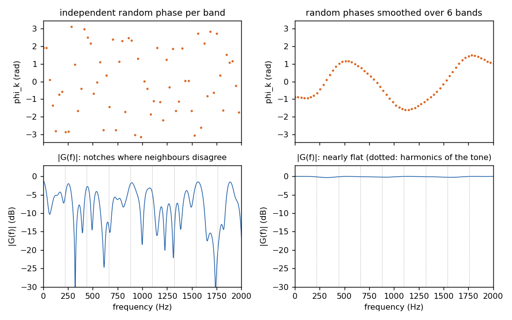
Figure 7. Left: independent random phases per band produce a magnitude response with deep notches. Right: the same random values smoothed over six bands give a nearly flat magnitude response. Dotted lines mark the harmonics of the tone.
Since the constant case is a filter, it does not need the filter bank at all: one could compute the FFT of the whole clip, multiply by exp(i phi(f)) for a smooth phase function, and invert. The filter bank version is equivalent, and we keep it because it also handles the time-varying case and because it displays the subband envelopes that the modification preserves.
6. Time-varying phase offsets are frequency modulation#
The app's cycling mode glides the phases from A to B and back. In the subband formulation this is phi_k(t) = s(t) delta_k with s a raised cosine. A phase that changes in time is indistinguishable from a change in frequency: the instantaneous frequency of band k is shifted by phi_k'(t) / (2 pi). Figure 8 plots this for a swing of pi radians at a cycle rate of 0.5 Hz, where the peak shift is about 0.8 Hz, and the peak shift as a function of cycle rate. Near 220 Hz the just noticeable difference in pitch is of the order of 1 Hz, so slow cycling is close to the threshold and fast cycling well above it. At 10 Hz the harmonics wobble by about 16 Hz, each by a different amount, so the tone is momentarily inharmonic and what is heard is vibrato and roughness rather than phase.
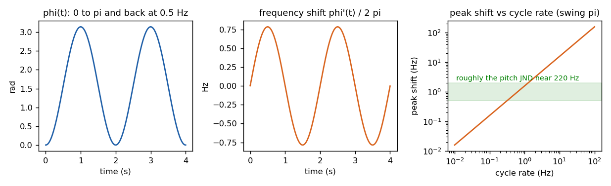
Figure 8. A raised-cosine phase offset (left), the frequency shift it implies (middle), and the peak shift as a function of cycle rate (right). The green band is roughly the pitch JND near 220 Hz.
This caveat applies to the existing cycling mode as much as to the extension. We therefore propose to keep phi_k(t) as a slow morph between two static maps, exactly as now, and to treat the cycle rate as something to keep low rather than as a free parameter to explore. Slowly varying offsets also keep the filter bank modification close to consistent, so the analysis of Section 5 applies at each instant.
7. Proposed app design#
Figure 9 summarizes the processing. Tone A is the original sound and tone B is the same sound with a phase map applied; both come out of the same filter bank, so they have the same subband envelopes at the chosen resolution.
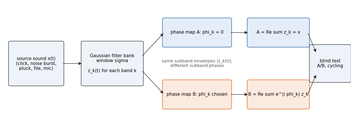
Figure 9. The proposed pipeline. A and B share every subband envelope and differ only in subband phase.
The controls we propose are the following.
- Source sound. A synthesized click, a noise burst, a plucked string (Karplus-Strong), and the existing harmonic tone cover the interesting cases and need no assets. A file loaded through
decodeAudioDataand a short microphone recording cover speech and music. - Window width sigma. A logarithmic slider from about 0.3 ms to 50 ms. This is the parameter that sets the group delay scale and hence the predicted audibility on transients.
- Phase map. A linear map phi_k = -2 pi f_k tau_0 is a pure delay and serves as a control that must be inaudible. A quadratic map is a chirp all-pass, the classic stimulus in the group delay literature. A random map smoothed over a chosen number of bands is the generic case. A per-harmonic map, for the tone source, reproduces the current app.
- Display. The waveforms of A and B, and their spectrograms recomputed at the analysis resolution, so the listener can see that the envelopes match while the waveforms differ. A plot of the group delay of the map, with the threshold band, states the prediction before listening.
- Listening. The existing play A then B, blind same/different test, and slow cycling.
Implementation is offline and fits the app's existing render-then-play design. For a clip of n samples, compute one FFT of length about 2n, and for each band multiply by the normalized Gaussian response, inverse transform, rotate by exp(i phi_k(t)), and accumulate the real part. With 256 bands and a two-second clip at 48 kHz this is a few hundred FFTs of length 2^18, on the order of a second in JavaScript, and it can run in a worker. The subband envelopes needed for the display come out of the same loop. The blind test component currently takes ToneParams for A and B; it would instead take two pre-rendered buffers, and the rest of it is unchanged. For the cycling mode, a real-time version would use a hop-based STFT with 75% overlap in an AudioWorklet and per-frame phase rotation, which is equivalent to the filter bank when the maps vary slowly. We suggest doing the offline version first.
8. Open questions and limitations#
The claim that A and B "have the same spectrogram" holds only at the analysis resolution, and Section 5 shows that the audible differences are exactly the ones visible at finer resolution. A more principled choice than a free window width would be a bank matched to auditory filters, with bandwidths that grow with frequency (an ERB-spaced gammatone bank). Under the hypothesis that the ear uses only subband envelopes at auditory resolution, phase rotation in such a bank should be inaudible for every sound, and finding an audible case would be informative. We suggest starting with the Gaussian bank because it is simpler and because the window width is then a single interpretable knob, and adding the auditory bank later.
The band at zero frequency and the smoothing at the ends of the map need care, and the choice of band spacing relative to bandwidth trades computation against how smooth the map must be. The group delay thresholds quoted above were measured with headphones and impulsive signals; over loudspeakers in a room the thresholds are higher because the room adds its own group delay. Finally, the extension does not change the basic statistics of the blind test, but with transient stimuli it will be important to randomize the interval between sounds so that timing cues do not leak information.